Transaction Prediction of Customers

Introduction.

In this project, A company wants to help them identify which customers will make a specific transaction in the future, irrespective of the amount of money transacted. The data provided for this project has the same structure as the real data they have available to solve this problem. The data is anonimyzed, each row containing 200 numerical values identified just with a number. In the following we will explore the data, prepare it for a model, train a model and predict the target value for the test set, then prepare a submission.

Prepare for Data Analysis.

Load Packages and Load data

Data Exploration

Check the Data

Let’s Check the test and train data.

Both train and test data have 200,000 entries and 202, respectivelly 201 columns.

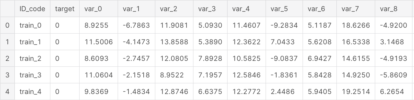
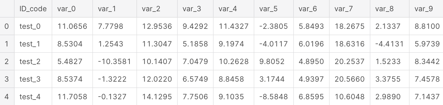
Let’s glimpse train and test dataset.

Basic Details

Train contains:

• ID_code (string);
• target;
• 200 numerical variables, named from var_0 to var_199;

Test contains:

• ID_code (string);
• 200 numerical variables, named from var_0 to var_199;
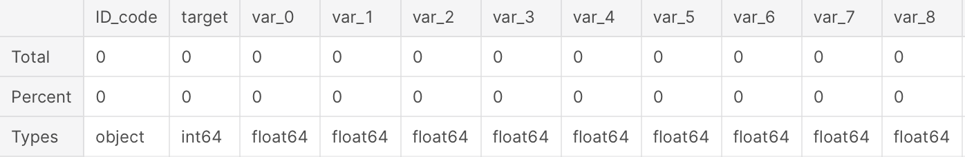
• Let’s check if there are any missing data. We will also check the type of data.

We check first train.

Here we check test dataset.

There are no missing data in train and test datasets. Let’s check the numerical values in train and test dataset.

Describe the Train Data

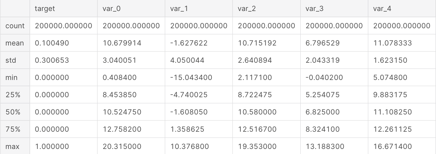
We can make few observations here:

• standard deviation is relatively large for both train and test variable data;
• min, max, mean, sdt values for train and test data looks quite close;
• mean values are distributed over a large range.

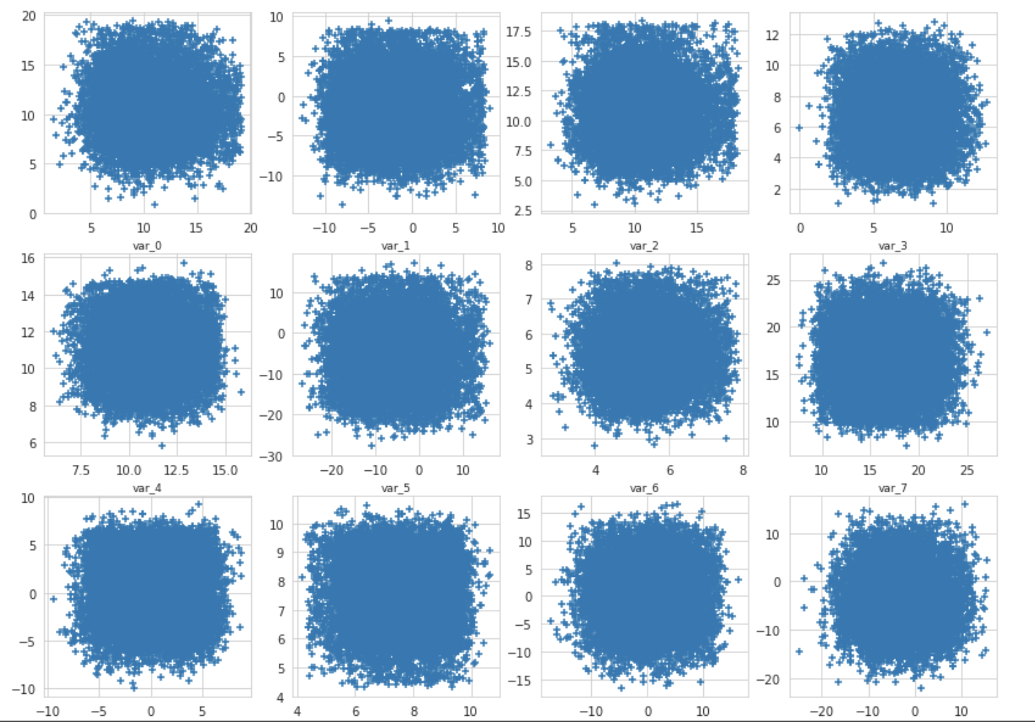
The number of values in train and test set is the same. Let’s plot the scatter plot for train and test set for few of the features.

We will show just 5% of the data. On x axis we show train values and on the y axis we show the test values.

Let’s check the distribution of target value in train dataset.

There are 10.049% target values with 1 The data is unbalanced with respect with target value.

Density plots of features.

Let’s show now the density plot of variables in train dataset.

We represent with different colors the distribution for values with target value 0 and 1.

t0 = train_df.loc[train_df['target'] == 0]
t1 = train_df.loc[train_df['target'] == 1]
features = train_df.columns.values[2:102]
plot_feature_distribution(t0, t1, '0', '1', features)

We can observe that there is a considerable number of features with significant different distribution for the two target values. For example, var_0, var_1, var_2, var_5, var_9, var_13, var_106, var_109, var_139 and many others.

Also some features, like var_2, var_13, var_26, var_55, var_175, var_184, var_196 shows a distribution that resambles to a bivariate distribution.

We will take this into consideration in the future for the selection of the features for our prediction model.

Le’t s now look to the distribution of the same features in parallel in train and test datasets.

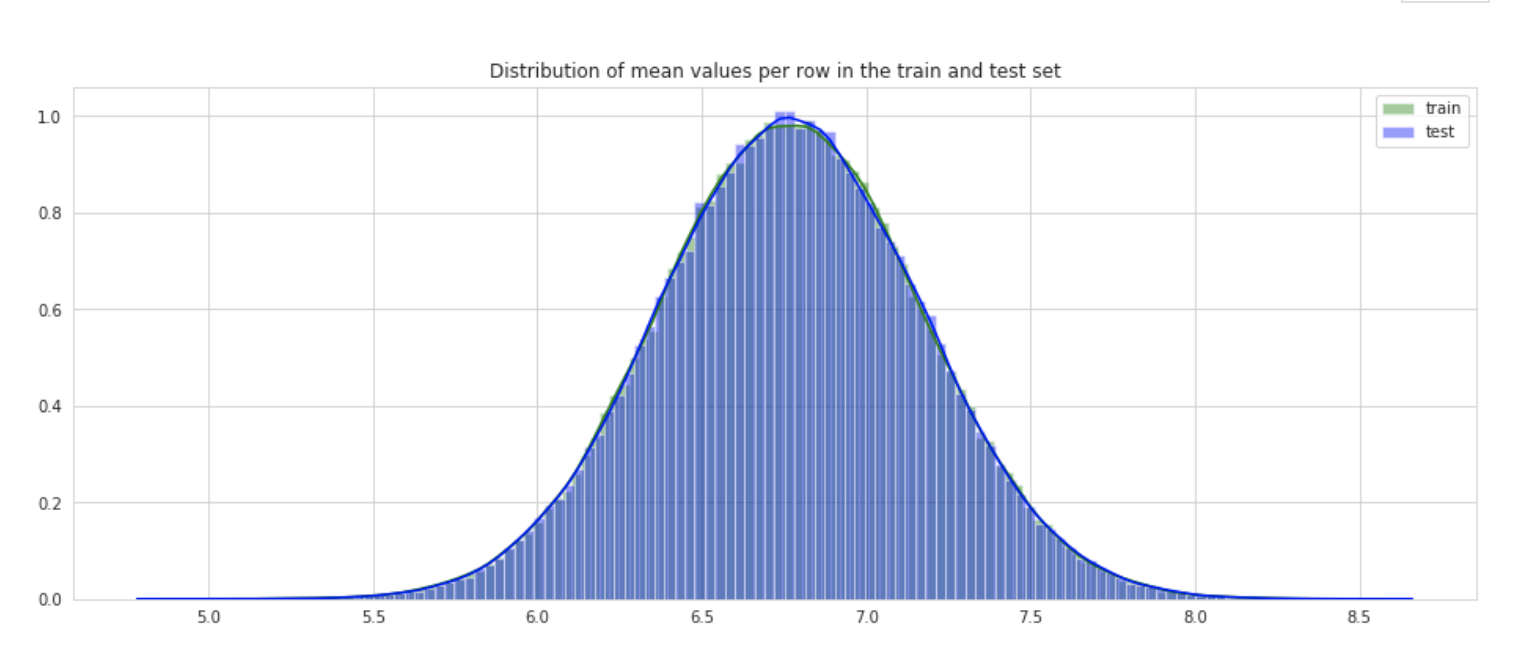
Distribution of mean and std

Let’s check the distribution of the mean values per row in the train and test set.

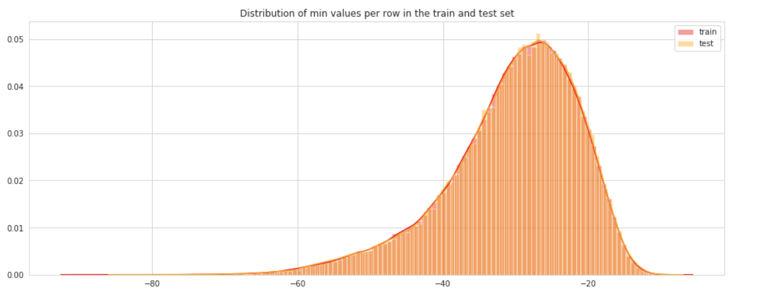
Distribution of min and max

Let’s check the distribution of min per row in the train and test set.

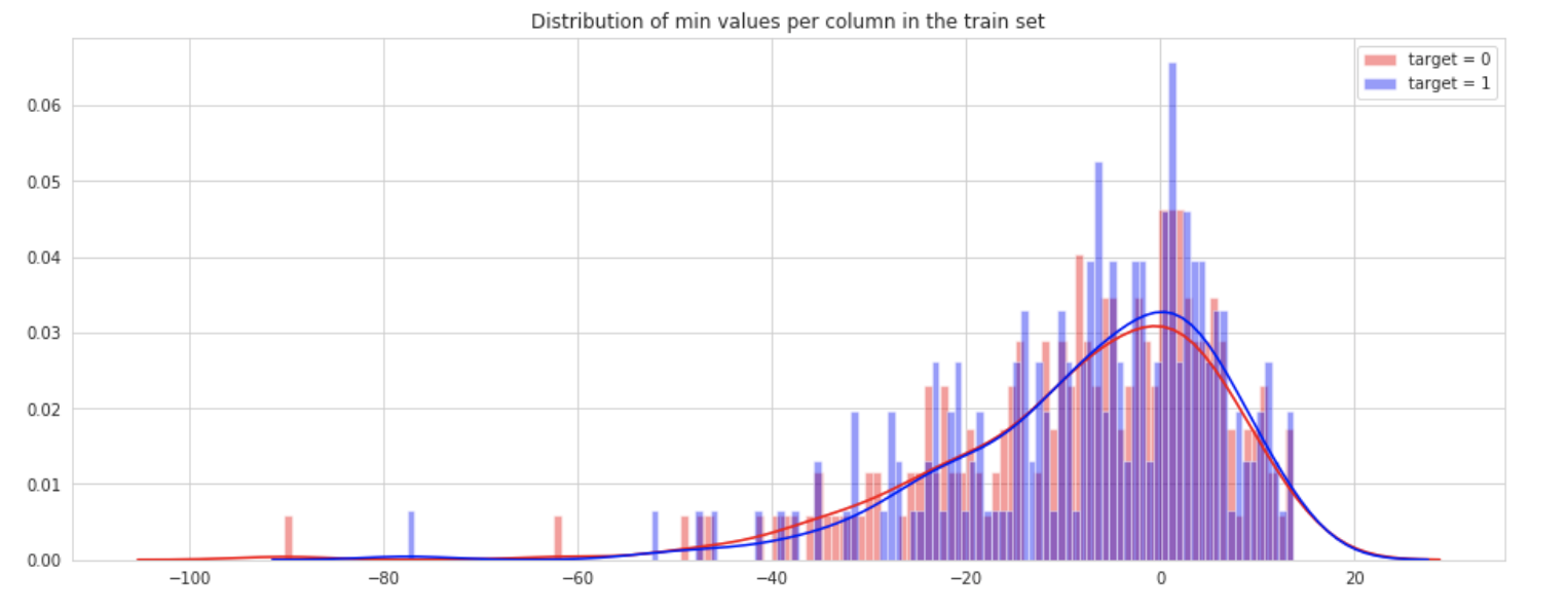
We show here the distribution of min values per columns in train set.

plt.figure(figsize=(16,6))
plt.title("Distribution of min values per column in the train set")
sns.distplot(t0[features].min(axis=0),color="red", kde=True,bins=120, label='target = 0')
sns.distplot(t1[features].min(axis=0),color="blue", kde=True,bins=120, label='target = 1')
plt.legend(); plt.show()

Distribution of skew and kurtosis

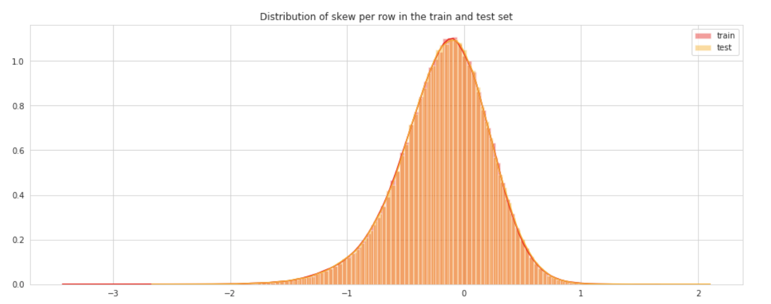
Let’s see now what is the distribution of skew values per rows and columns.

Let’s see first the distribution of skewness calculated per rows in train and test sets.

Features correlation

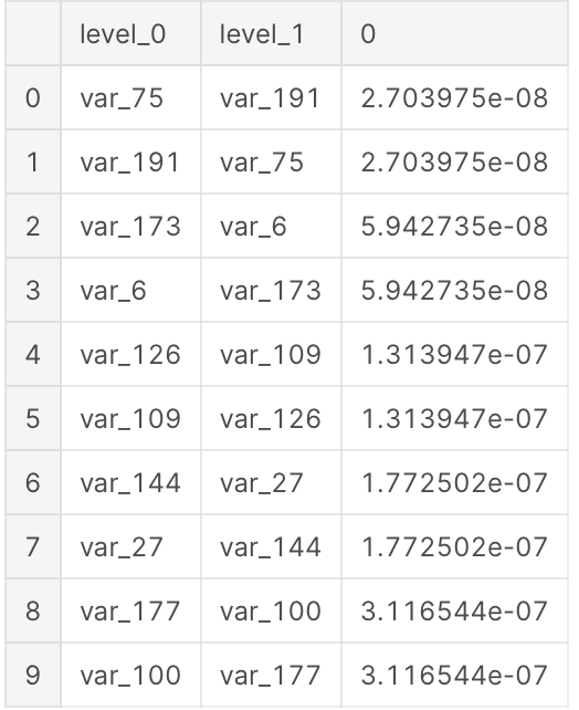
We calculate now the correlations between the features in train set. The following table shows the first 10 the least correlated features.

correlations = train_df[features].corr().abs().unstack().sort_values(kind="quicksort").reset_index()
correlations = correlations[correlations['level_0'] != correlations['level_1']]
correlations.head(10)

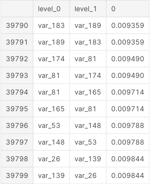
Let’s look to the top most correlated features, besides the same feature pairs.

Let’s see also the least correlated features.

Feature engineering

Let’s calculate for starting few aggregated values for the existing features.

idx = features = train_df.columns.values[2:202]
for df in [test_df, train_df]:
    df['sum'] = df[idx].sum(axis=1)  
    df['min'] = df[idx].min(axis=1)
    df['max'] = df[idx].max(axis=1)
    df['mean'] = df[idx].mean(axis=1)
    df['std'] = df[idx].std(axis=1)
    df['skew'] = df[idx].skew(axis=1)
    df['kurt'] = df[idx].kurtosis(axis=1)
    df['med'] = df[idx].median(axis=1)

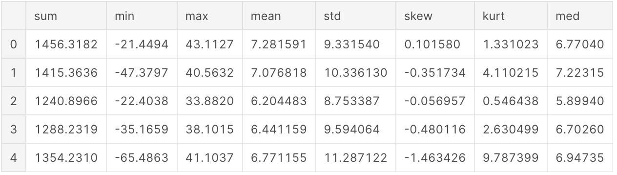
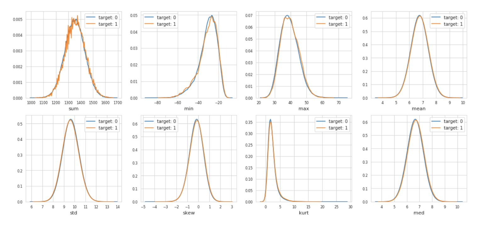
Let’s check the distribution of these new, engineered features.

We plot first the distribution of new features, grouped by value of corresponding target values.

t0 = train_df.loc[train_df['target'] == 0]
t1 = train_df.loc[train_df['target'] == 1]
features = train_df.columns.values[202:]
plot_new_feature_distribution(t0, t1, 'target: 0', 'target: 1', features)

Model

From the train columns list, we drop the ID and target to form the features list.

features = [c for c in train_df.columns if c not in ['ID_code', 'target']]
target = train_df['target']

We define the hyperparameters for the model.

param = {
    'bagging_freq': 5,
    'bagging_fraction': 0.4,
    'boost_from_average':'false',
    'boost': 'gbdt',
    'feature_fraction': 0.05,
    'learning_rate': 0.01,
    'max_depth': -1,  
    'metric':'auc',
    'min_data_in_leaf': 80,
    'min_sum_hessian_in_leaf': 10.0,
    'num_leaves': 13,
    'num_threads': 8,
    'tree_learner': 'serial',
    'objective': 'binary',
    'verbosity': 1
}

We run the model.

folds = StratifiedKFold(n_splits=10, shuffle=False, random_state=44000)
oof = np.zeros(len(train_df))
predictions = np.zeros(len(test_df))
feature_importance_df = pd.DataFrame()

for fold_, (trn_idx, val_idx) in enumerate(folds.split(train_df.values, target.values)):
    print("Fold {}".format(fold_))
    trn_data = lgb.Dataset(train_df.iloc[trn_idx][features], label=target.iloc[trn_idx])
    val_data = lgb.Dataset(train_df.iloc[val_idx][features], label=target.iloc[val_idx])

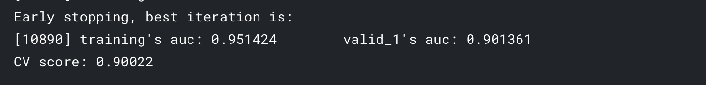
    num_round = 1000000
    clf = lgb.train(param, trn_data, num_round, valid_sets = [trn_data, val_data], verbose_eval=1000, early_stopping_rounds = 3000)
    oof[val_idx] = clf.predict(train_df.iloc[val_idx][features], num_iteration=clf.best_iteration)

    fold_importance_df = pd.DataFrame()
    fold_importance_df["Feature"] = features
    fold_importance_df["importance"] = clf.feature_importance()
    fold_importance_df["fold"] = fold_ + 1
    feature_importance_df = pd.concat([feature_importance_df, fold_importance_df], axis=0)

    predictions += clf.predict(test_df[features], num_iteration=clf.best_iteration) / folds.n_splits

print("CV score: {:<8.5f}".format(roc_auc_score(target, oof)))

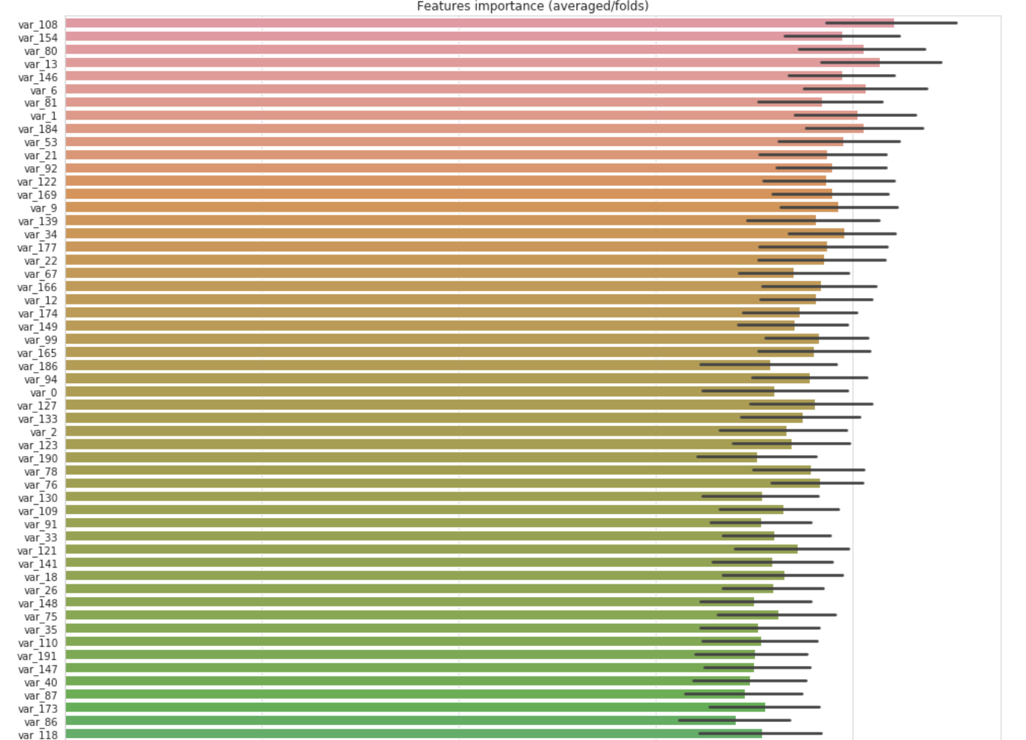
Let’s check the feature importance.

cols = (feature_importance_df[["Feature", "importance"]]
        .groupby("Feature")
        .mean()
        .sort_values(by="importance", ascending=False)[:150].index)
best_features = feature_importance_df.loc[feature_importance_df.Feature.isin(cols)]

plt.figure(figsize=(14,28))
sns.barplot(x="importance", y="Feature", data=best_features.sort_values(by="importance",ascending=False))
plt.title('Features importance (averaged/folds)')
plt.tight_layout()
plt.savefig('FI.png')

Code

Thank you for reading