

SVM Classification - Credit Card
Introduction
In this kernel we will use various predictive models to see how accurate they are in detecting whether a transaction is a normal payment or a fraud. As described in the dataset, the features are scaled and the names of the features are not shown due to privacy reasons. Nevertheless, we can still analyze some important aspects of the dataset. Let’s start!
Importing Libraries
import pandas as pd
import numpy as np

# Scikit-learn library: For SVM
from sklearn import preprocessing
from sklearn.metrics import confusion_matrix
from sklearn import svm

import itertools

# Matplotlib library to plot the charts
import matplotlib.pyplot as plt
import matplotlib.mlab as mlab

# Library for the statistic data vizualisation
import seaborn

%matplotlib inline
Data Recuperation
data = pd.read_csv('../input/creditcard.csv') # Reading the file .csv
df = pd.DataFrame(data) # Converting data to Panda DataFrame
Data Visualization
df = pd.DataFrame(data) # Converting data to Panda DataFrame
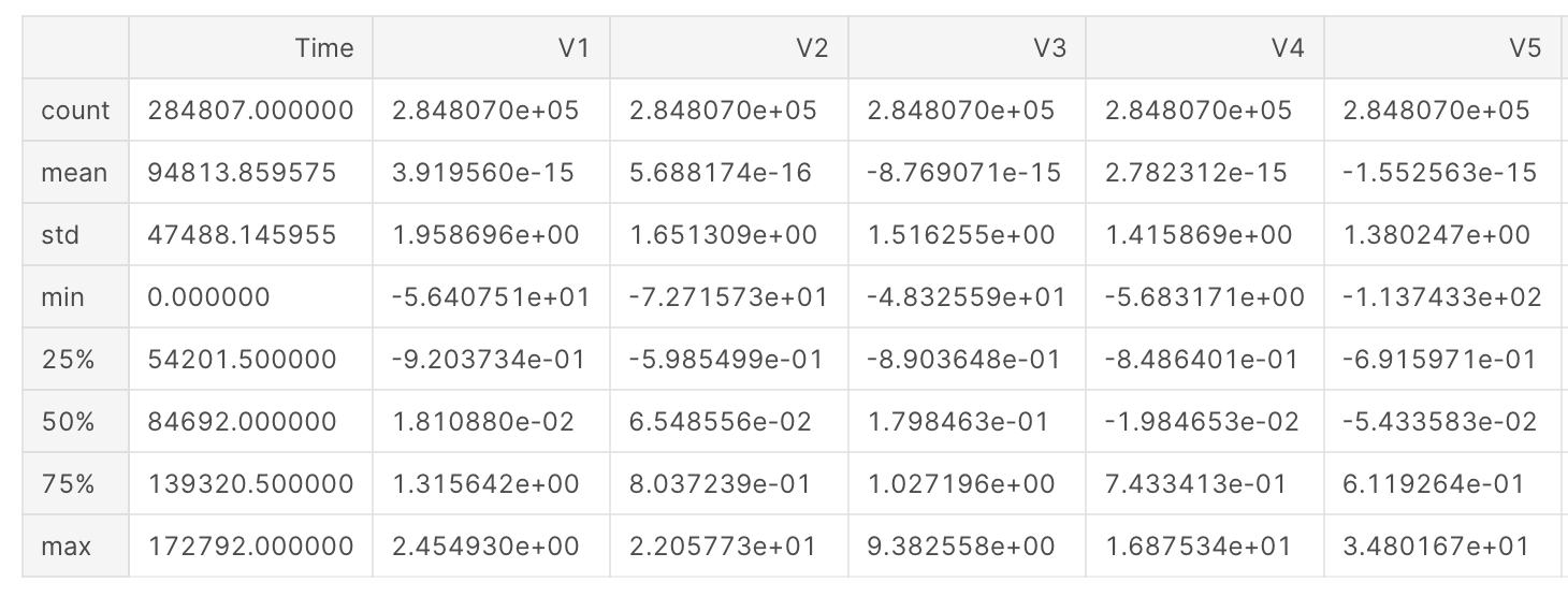
df.describe() # Description of statistic features (Sum, Average, Variance, minimum, 1st quartile, 2nd quartile, 3rd Quartile and Maximum)
df_fraud = df[df['Class'] == 1] # Recovery of fraud data
plt.figure(figsize=(15,10))
plt.scatter(df_fraud['Time'], df_fraud['Amount']) # Display fraud amounts according to their time
plt.title('Scratter plot amount fraud')
plt.xlabel('Time')
plt.ylabel('Amount')
plt.xlim([0,175000])
plt.ylim([0,2500])
plt.show()
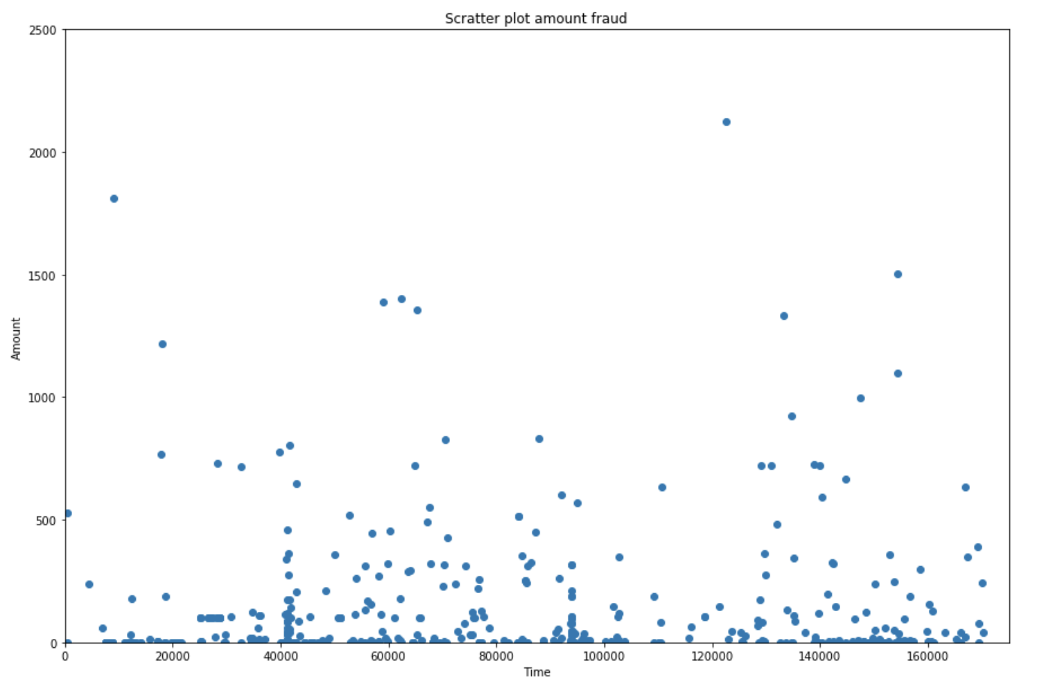
nb_big_fraud = df_fraud[df_fraud['Amount'] > 1000].shape[0] # Recovery of frauds over 1000
print('There are only '+ str(nb_big_fraud) + ' frauds where the amount was bigger than 1000 over ' + str(df_fraud.shape[0]) + ' frauds')
There are only 9 frauds where the amount was bigger than 1000 over 492 frauds
Unbalanced Data
number_fraud = len(data[data.Class == 1])
number_no_fraud = len(data[data.Class == 0])
print('There are only '+ str(number_fraud) + ' frauds in the original dataset, even though there are ' + str(number_no_fraud) +' no frauds in the dataset.')
There are only 492 frauds in the original dataset, even though there are 284315 no frauds in the dataset. This dataset is unbalanced which means using the data as it is might result in unwanted behaviour from a supervised classifier. To make it easy to understand if a classifier were to train with this data set trying to achieve the best accuracy possible it would most likely label every transaction as a non-fraud.
Correlation of Features
df_corr = df.corr() # Calculation of the correlation coefficients in pairs, with the default method:
                    # Pearson, Standard Correlation Coefficient
In [10]:
plt.figure(figsize=(15,10))
seaborn.heatmap(df_corr, cmap="YlGnBu") # Displaying the Heatmap
seaborn.set(font_scale=2,style='white')

plt.title('Heatmap correlation')
plt.show()
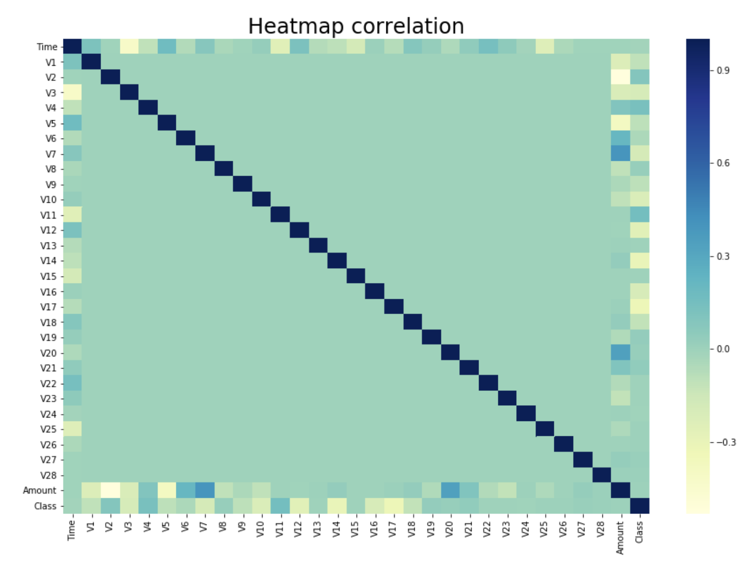
As we can notice, most of the features are not correlated with each other. This corroborates the fact that a PCA was previously performed on the data.
What can generally be done on a massive dataset is a dimension reduction. By picking th emost important dimensions, there is a possiblity of explaining most of the problem, thus gaining a considerable amount of time while preventing the accuracy to drop too much.
However in this case given the fact that a PCA was previously performed, if the dimension reduction is effective then the PCA wasn’t computed in the most effective way. Another way to put it is that no dimension reduction should be computed on a dataset on which a PCA was computed correctly.
rank = df_corr['Class'] # Retrieving the correlation coefficients per feature in relation to the feature class
df_rank = pd.DataFrame(rank)
df_rank = np.abs(df_rank).sort_values(by='Class',ascending=False) # Ranking the absolute values of the coefficients
                                                                  # in descending order
df_rank.dropna(inplace=True) # Removing Missing Data (not a number)
Confusion Matrix
class_names=np.array(['0','1']) # Binary label, Class = 1 (fraud) and Class = 0 (no fraud)
In [18]:
# Function to plot the confusion Matrix
def plot_confusion_matrix(cm, classes,
                          title='Confusion matrix',
                          cmap=plt.cm.Blues):

    plt.imshow(cm, interpolation='nearest', cmap=cmap)
    plt.title(title)
    plt.colorbar()
    tick_marks = np.arange(len(classes))
    plt.xticks(tick_marks, classes, rotation=45)
    plt.yticks(tick_marks, classes)

    fmt = 'd'
    thresh = cm.max() / 2.
    for i, j in itertools.product(range(cm.shape[0]), range(cm.shape[1])):
        plt.text(j, i, format(cm[i, j], fmt),
                 horizontalalignment="center",
                 color="white" if cm[i, j] > thresh else "black")

    plt.tight_layout()
    plt.ylabel('True label')
    plt.xlabel('Predicted label')
Model Selection
classifier = svm.SVC(kernel='linear') # We set a SVM classifier, the default SVM Classifier (Kernel = Radial Basis Function)
In [20]:
classifier.fit(X_train, y_train) # Then we train our model, with our balanced data train.
SVC(C=1.0, cache_size=200, class_weight=None, coef0=0.0, decision_function_shape=’ovr’, degree=3, gamma=’auto’, kernel=’linear’, max_iter=-1, probability=False, random_state=None, shrinking=True, tol=0.001, verbose=False)
Testing the Model
prediction_SVM_all = classifier.predict(X_test_all) #And finally, we predict our data test.
In [22]:
cm = confusion_matrix(y_test_all, prediction_SVM_all)
plot_confusion_matrix(cm,class_names)
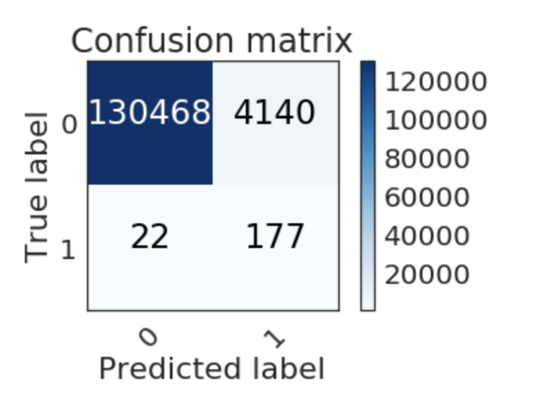
In this case we are gonna try to minimize the number of errors in our prediction results. Errors are on the anti-diagonal of the confusion matrix. But we can infer that being wrong about an actual fraud is far worse than being wrong about a non-fraud transaction.
That is why using the accuracy as only classification criterion could be considered unthoughtful. During the remaining part of this study our criterion will consider precision on the real fraud 4 times more important than the general accuracy. Even though the final tested result is accuracy.
We have detected 177 frauds / 199 total frauds.
So, the probability to detect a fraud is 0.889447236181 the accuracy is : 0.969126232317